The calculation table is very important in sensors configuration (see sensor properties). According to the calculation table adjusted, raw data coming in a parameter is transformed into sensor values, for instance, some abstract 86 is interpreted as 10.5 liters of fuel.
The calculation table is not always necessary. For example, if the sensor is digital and sends only 1 or 0, which correspond to the On/Off states, there is no need in the value calculation table for such a sensor.
The completed calculation table is essential for the analog engine ignition sensor since it is necessary to determine how all available analog values are transformed into two available states — On/Off.
Calculation table recalculates data according to to the equation of the straight line Y = a×X + b, where:
X is the input value that comes from the device;
Y is the output value that is included in the reports, charts, tooltips, etc.;
a is the coefficient that determines the slope or gradient of the line (tangent of the angle, or relation of the opposite cathetus to the adjoining one);
b is the displacement of a straight line along the Y-axis.
Upon the arrival of the value (i.e. X), it is substituted into the calculation table, a and b are calculated automatically, and the output receives a final value, i.e. Y (it gets into reports, graphs, tooltips, etc.).
Each row of the table operates only within its segment that is to the X value of the next row. That is why X values cannot be repeated.
It is possible to get the tangent of the angle (that is needed to be substituted for the a coefficient) using mathematics. To do it, find on the X and Y axes the segments of values operation (deltas). Then divide the values ∆y/∆x. The result value is the tangent of the angle.
Lower and upper bounds are used to set the limits for input values. Note that the bounds correspond to the half-open interval. In other words, the lower bound is included in the interval of valid values while the upper one is not. In case of receiving values beyond the indicated interval, these values are considered to be invalid. Moreover, depending on the enabling/disabling of the Apply after calculation checkbox, the indicated limits are applied to the raw values X (disabled checkbox), or to the processed values Y (enabled checkbox).
Incorrect pairs of values can be removed with the button . To remove all pairs at once, click on the delete button in the header of the table.
A graphic for the created calculation table can be viewed by clicking the Show chart icon at the top of the table header.
Methods of filling the table
Fill in all available fields (X, b, and a). Use this method to get the calculation table under your complete control.
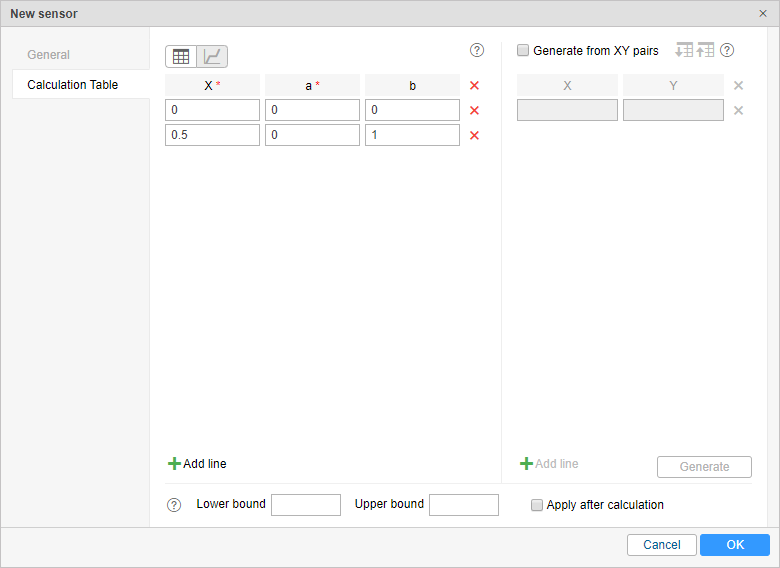
Fill in only X and b values, and a set as zero. This method is convenient if you need to convert an analog signal to a digital one.
Fill in only X and a values. In this case, b is calculated automatically. This method is convenient if you need to get a curve knowing the angles, but without recalculating the Y offset.
In some cases, it is possible to adjust the calculation table knowing the X and Y values. In such cases use the calculation table wizard (right part of the dialog box).
Chart managing
A chart can be managed using the following buttons:
Area selection | When this button is activated, it becomes possible to scale (zoom) any selected area of the chart. To do this, select the appropriate area by holding the left mouse button. The procedure can be repeated any number of times. |
Autoscaling | This button allows you to return to the default chart scale. |
/ Zoom in/zoom out | The buttons to scale a chart along the X-axis. Click on the button in order to make the visible area of the chart twice as wide/narrow in regards to the current position. Yet the center of the chart stays in its place. |
Save as PNG | This button allows you to save the visible chart area along with the axis in PNG format. |
Example 1: temperature sensor
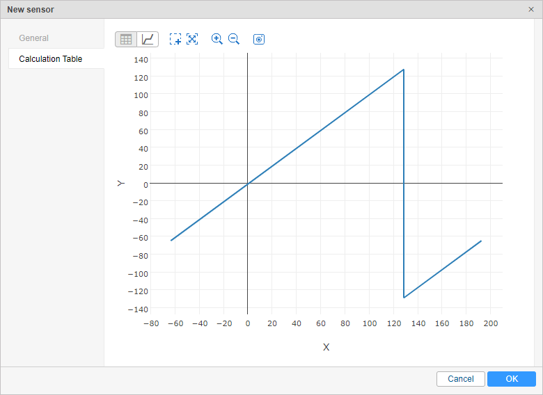
As an example, let us create a calculation table for the temperature sensor. Suppose that the data is coming in complement code, i. e. the positive values are from 0 to 127, and negative from 128 (which corresponds to -128 degrees) to 255 (which corresponds to -1 degree).
On the basis of the values indicated in the table, a chart is made. To view the chart, click the Show chart icon.
The calculation graph always has a somewhat extended view — along the X-axis it stretches to the right and to the left. This is due to the fact that on the first interval the function also works in the opposite direction — up to minus infinity, and on the last interval — up to plus infinity.
Example 2: engine ignition sensor
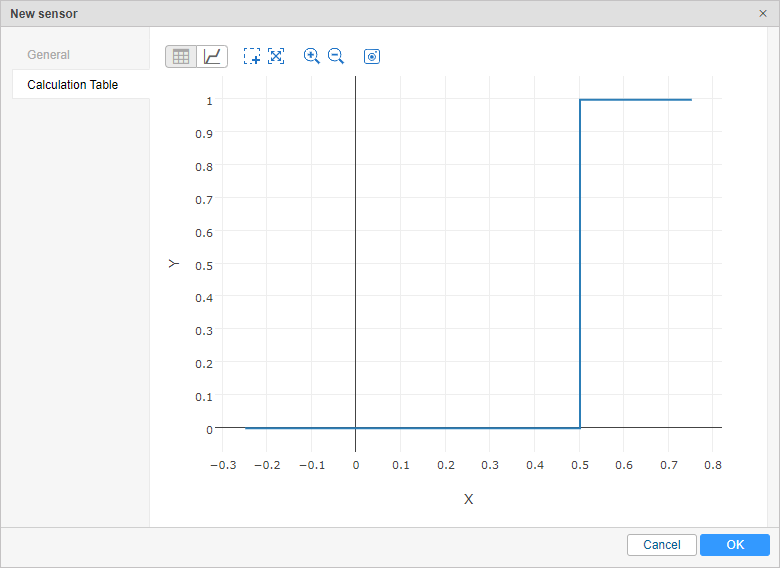
It is possible to configure a non-digital ignition sensor based on the parameter sending voltage. For instance, the voltage up to 0.5 V would mean ignition off, and over 0.5 V — ignition on. For such a sensor, we should create a calculation table as shown above:
Move to the Calculation chart and see if the result meets your expectations.
Calculation table wizard
The Calculation Table Wizard is a tool that simplifies the process of creating a calculation table. It is sufficient to indicate input X values and corresponding output Y values. You can use the calculation table wizard to calibrate a sensor experimentally. For instance, you fill in different volumes of fuel into the tank and each time you take the readings from the sensor. The Calculation Table Wizard is located on the right side of the dialog window. It is disabled by default. To use a wizard, indicate the Generate from XY pairs flag.
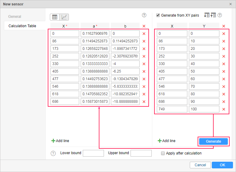
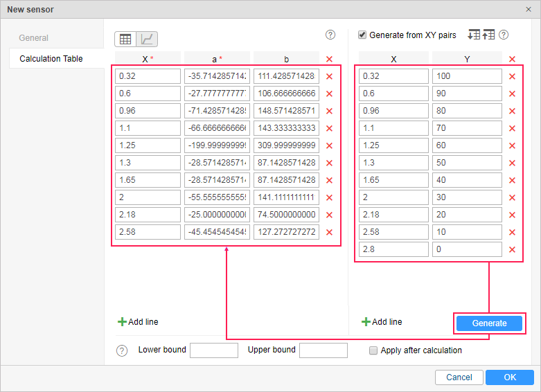
Enter the pairs and click Generate in order for them to be processed by the system. On the basis of values indicated in the wizard, a calculation table will be created.
The program calculates a and b using the following algorithm.
a is calculated by the formula ∆Y/∆X. X- and Y-axial displacement is calculated separately for each interval, and then Y-axial displacement is divided by X-axial displacement, that is ∆Y/∆X.
b is calculated by the formula b = Y — a × X.
In the upper right corner of the table wizard, there are buttons for exporting the introduced XY pairs into a CSV file and importing values from CSV or TXT files.
Example 1: fuel level sensor
Suppose that 10 liters of fuel was filled and the sensor sent the value 86, then 20 liters were added and the sensor showed 173, and so on. In the end, we can form a table:
Input values (X) | Output values (Y) |
|---|---|
0 | 0 |
86 | 10 |
173 | 20 |
252 | 30 |
330 | 40 |
405 | 50 |
477 | 60 |
546 | 70 |
618 | 80 |
686 | 90 |
749 | 100 |
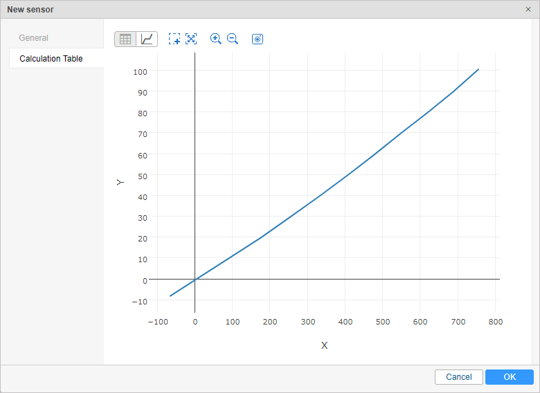
Enter these pairs into the wizard and click Generate. Based on the entered values, a calculation table (on the left) is generated.
In order to view a chart, click the Show chart icon.
All the data entered and saved on this tab is available when you open the dialog. Any changes in the calculation table do not affect the Wizard. In other words, the Wizard only shows the entered values but does not reflect the current situation.
Now let us see how a and b were calculated. The first interval starts with 0 and lasts until 86. At that, at the last point the output is 10. So, X displacement is ∆Х = 86 — 0 = 86, and Y displacement is ∆Y = 10 — 0 = 10. Now a coefficient can be calculated: a = ∆Y/∆X = 10 / 86 = 0,11627906976744186.
For other intervals, we apply the same calculation scheme (there will be one interval less than there are rows in the Calculation Wizard):
Interval | X | Y | a | b |
|---|---|---|---|---|
N | X | Y | (Y(i+1) — Y(i)) / (X(i+1) — X(i)) | Y — a × X |
1 | 0 | 0 | (10 — 0) / (86 — 0) | 0 — a×0 |
2 | 86 | 10 | (20 — 10) / (173 — 86) | 10 — a×86 |
3 | 173 | 20 | (30 — 20) / (252 — 173) | 20 — a×173 |
4 | 252 | 30 | (40 — 30) / (330 — 252) | 30 — a×252 |
5 | 330 | 40 | (50 — 40) / (405 — 330) | 40 — a×330 |
6 | 405 | 50 | (60 — 50) / (477 — 405) | 50 — a×405 |
7 | 477 | 60 | (70 — 60) / (546 — 477) | 60 — a×477 |
8 | 546 | 70 | (80 — 70) / (618 — 546) | 70 — a×546 |
9 | 618 | 80 | (90 — 80) / (686 — 618) | 80 — a×618 |
10 | 686 | 90 | (100 — 90) / (749 — 686) | 90 — a×686 |
11 | 749 | 100 | (110 — 100) / (812 — 749) | 100 — a×749 |
The information on how to make the calibration of a fuel tank can be found here.
Example 2: fuel level sensor
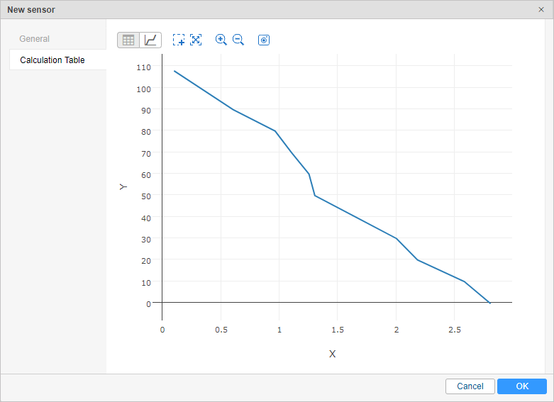
In this example, input X values decline while output Y values grow. Insert the pairs into the Wizard in any order — they will be rearranged automatically.
Initial data:
Input values (X) | Output values (Y) |
|---|---|
2.8 | 0 |
2.58 | 10 |
2.18 | 20 |
2.0 | 30 |
1.65 | 40 |
1.3 | 50 |
1.25 | 60 |
1.1 | 70 |
0.96 | 80 |
0.6 | 90 |
0.32 | 100 |
Enter these pairs into the Wizard, generate the calculation table and view the calculation chart.
Calculated intervals for this sensor are as follows:
Interval | X | Y | a | b |
|---|---|---|---|---|
N | X | Y | (Y(i+1) — Y(i)) / (X(i+1) — X(i)) | Y — a × X |
1 | 0,32 | 100 | (90 — 100) / (0,6 — 0,32) | 100 — a×0,32 |
2 | 0,6 | 90 | (80 — 90) / (0,96 — 0,6) | 90 — a×0.6 |
3 | 0,96 | 80 | (70 — 80) / (1,1 — 0,96) | 80 — a×0.96 |
4 | 1,1 | 70 | (60 — 70) / (1,25 — 1,1) | 70 — a×1.1 |
5 | 1,25 | 60 | (50 — 60) / (1,3 — 1,25) | 60 — a×1.25 |
6 | 1,3 | 50 | (40 — 50) / (1,65 — 1,3) | 50 — a×1.3 |
7 | 1,65 | 40 | (30 — 40) / (2,0 — 1,65) | 40 — a×1.65 |
8 | 2,0 | 30 | (20 — 30) / (2,18 — 2,0) | 30 — a×2 |
9 | 2,18 | 20 | (10 — 20) / (2,58 — 2,18) | 20 — a×2.18 |
10 | 2,58 | 10 | (0 — 10) / (2,8 — 2,58) | 10 — a×2.58 |
The information on how to make the calibration of a fuel tank can be found here.


