Sensors: Calculation table explained
One of the first and crucial stages of working with Wialon is setting up sensors in the unit. If the sensors are set up correctly, then some standard algorithms will give more accurate results and you will get access to functionality that has not been available before. The calculation table, a tool from the tab of the same name, is considered in detail in this article since this exact tool most often causes difficulties when setting up sensors.
The article contains information of varying complexity. The main part is helpful for understanding the logic of the calculation table. However, you can find more detailed mathematical formulations in the highlighted special blocks called It’s Math Time. For a general understanding of this article, you can skip these blocks.
General principle of sensors operation
Wialon supports many types of trackers; you can find their current number on the wialon.com website in the Hardware section. Each of the trackers “speaks” in its own way. Therefore, the parameters which come from different types of trackers and which are displayed on the Messages tab may contain the same information (for example, about temperature or mileage) but have different names. It is necessary to create sensors for each unit in Wialon to prevent users from noticing the differences when using units with various trackers. Also, sensors have a specific type, which allows the system to understand which algorithm to choose to process input values.
However, a simple selection of a sensor type and specifying a parameter in it is often not enough because the parameter value comes in an unobvious to the user way. For example, temp=125 could mean 125°F, 125°C, 12.5°C, or even -3°C. There are three methods to convert the input parameter to the desired type:
- Expression in the Parameter field;
- Calculation table;
- Validation.
They can be used individually or combined. If you use several methods simultaneously, they will be applied in the exact order they are listed above.
Schematically, the use of sensors can be represented as follows:
- The sensor connected to the tracker measures some physical quantity; let’s denote it by S.
- The sensor converts this value and transmits it to the tracker. The X parameter comes from the tracker to Wialon.
- Based on the parameter, a sensor is created in Wialon. Then, f(X) transformations are applied to the parameter in the sensor to obtain a human-readable Y value.
- Ideally, after transformations in the sensor, the value Y=f(X) should be equal to the value S measured in the first stage. Further, Y will be used in tooltips, reports, notifications, and other Wialon functionality.
![]()
Since this article only explains the process of setting up the calculation table in Wialon, we will pay attention only to the following elements from the scheme above:
![]()
When to use a calculation table
Usually, the calculation table is used in cases where it is necessary to convert the input parameter. However, all three methods mentioned above serve to do this. In what scenario is it worth choosing the calculation table?
In terms of practical application, the calculation table might be used for:
- the calibration table (for example, for weight sensors or fuel level sensors);
- digital sensors based on analog input data (for example, ignition sensors based on voltage);
- sensors based on codes that describe different states but come in one parameter (for example, device_status=4 means the ignition is on, and device_status=13 means the panic button is pressed, etc.);
- sensors that should display positive and negative values, although the parameter associated with them has only positive values (for example, for temperature sensors);
- any sensors in which it is necessary to separate the range of correct and erroneous values (for example, if the sensor sends specific values in a parameter that indicate errors).
Calculation table settings
The calculation table involves working with the simplest linear functions. That means that the calculation table converts the data in accordance with the Y=a⋅X+b formula — one of the variants of the straight-line equation.
If you understand how each component of this equation works, you can implement valuable and unusual solutions with its help. Next, we will review each area of the Calculation Table tab separately and visualize its impact on the result using a chart.
To see a chart that corresponds to the completed calculation table, you need to click on the icon ![]() at the top of the tab.
at the top of the tab.
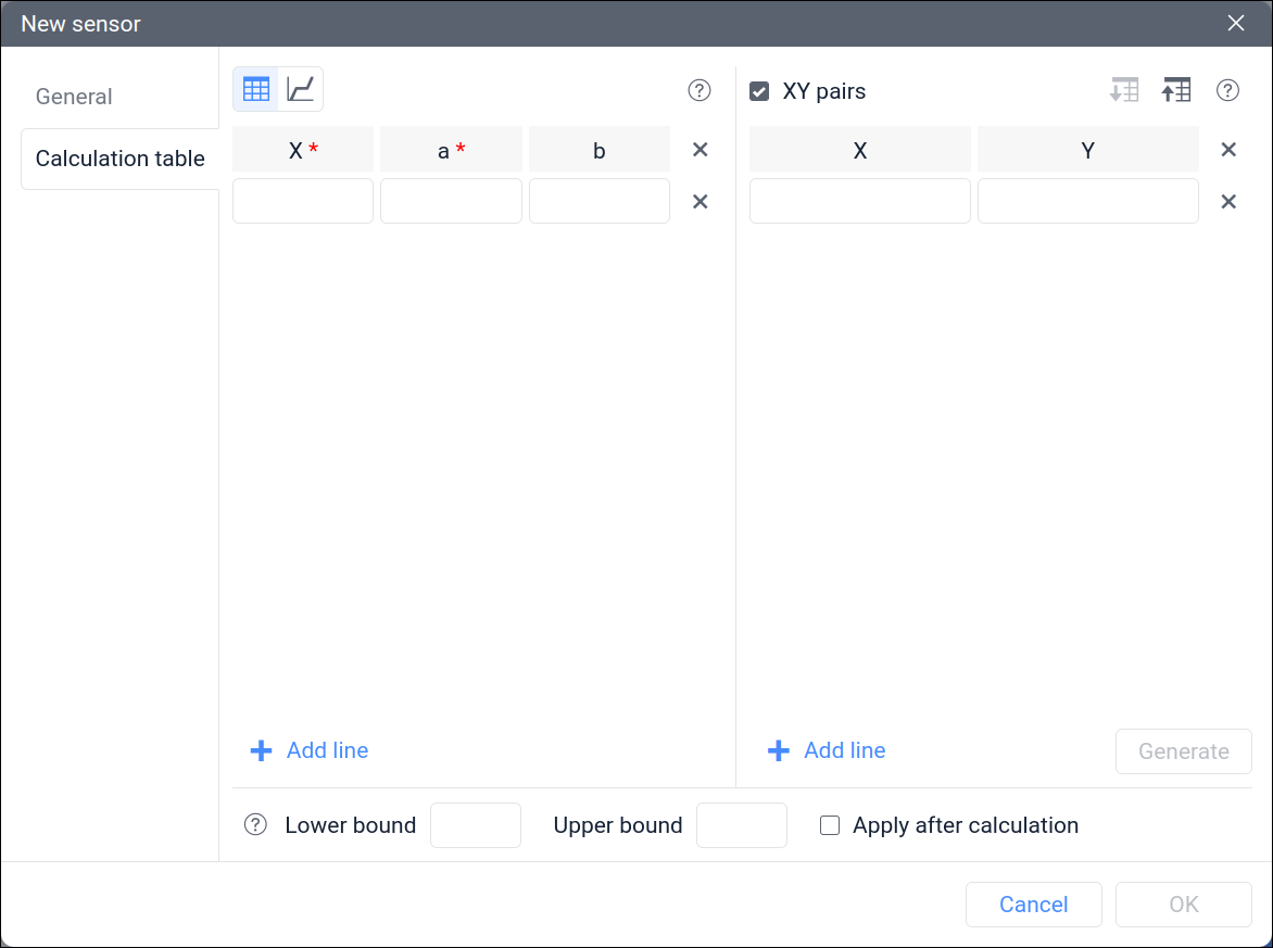
XY pairs
On the right side, you can see the XY pairs block. Filling it in is not enough for the calculation table to work, but it can simplify its settings.
We recommend using XY pairs only for fuel level sensors to add the calibration table. In other cases, you should independently calculate and enter the values of X, a, and b.
You can add pairs manually or by importing CSV or TXT files (export is available in CSV only). After filling in all the fields of this block, you must click the Generate button (meaning, generate a calculation table based on XY pairs). This action will lead to the values of X, a, and b calculation in the left part of the window.
Each of the added XY pairs corresponds to a point on the chart. As you know, you can draw a line through two points. Therefore, if you enter five XY pairs, you will get four straight lines on the chart.
Pairs with the same X value are not allowed to enter. This is technically impossible since two or more Y values cannot correspond to one X value. However, you can enter the same Y values.
X is an input value
The central block of the Calculation Table tab contains rows with X, a, and b values. Each of the rows corresponds to a straight line on the chart. The value of X in each row means the beginning of a new straight line, that is, it sets the interval where new values of a and b will be used.
The last row affects all further values up to +∞, and the first row affects values even up to the first specified X, i.e., starting from −∞. Therefore, writing several consecutive rows with the same values of a and b does not make sense.
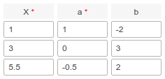
As an example, consider a table with the following values:
Otherwise, this condition can be written as follows:
- From −∞ to 3 (not including), the equation Y=1⋅X-2 is applied.
- From 3 (including) to 5.5 (not including), the equation Y=0⋅X+3 is applied.
- From 5.5 (including) to +∞, the equation Y=-0.5⋅X+2 is applied.
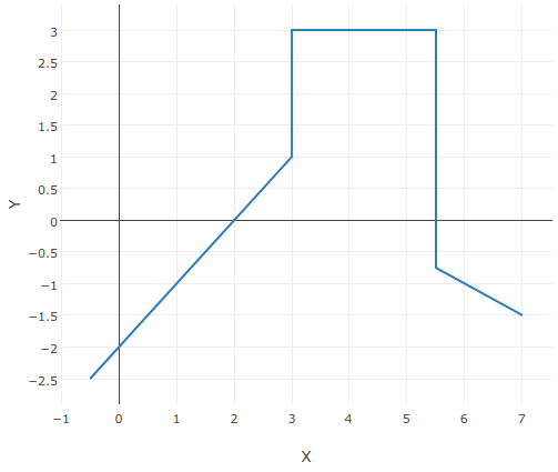
An example of a chart obtained when filling in the calculation table
a is a slope coefficient of the line
With a=0, the slope will be 0°; thus, the line will be parallel to the X-axis.
With a=1, the slope will be 45°; thus, the larger the coefficient, the closer the line will be to the Y-axis.
With a=-1, the slope will be −45 °; thus, negative values of this coefficient tilt the line down, and positive values — up.
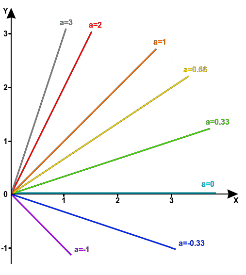
An example of a chart of the Y=a⋅X line with different slope coefficients
Determining the coefficient of the line slope is quite simple: its value equals the ratio of the change in Y to the change in X.
As an example, consider the green line in the chart above. It shows that Y increases from 0 to 1 when X grows from 0 to 3, which means that the coefficient for this line is a=(1-0)/(3-0)=1/3=0.33.
b determines the displacement of the line along the Y-axis
When b=0, there is no displacement.
When b>0, the straight line is displaced upward relative to the X-axis.
When b<0, the displacement is downward.
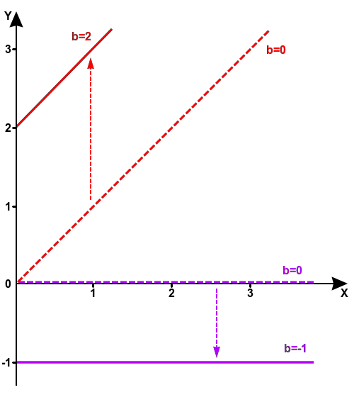
An example of lines with different displacements
When using XY pairs, the value of b is automatically calculated so that the next line segment smoothly continues the previous one.
Calculating the value of b is not as simple as the slope coefficient since usually it has no clear analogy outside of mathematics other than the displacement of the line up or down.
The only exception is when a digital sensor is set up using the calculation table. In this case, a=0, and the formula becomes Y=b. Therefore, the value of b will be equal to what you expect to see as Y.
Lower and upper bounds
Lower and upper bounds allow you to cut off erroneous sensor values according to a simple principle — if the value is outside the range between the lower and upper bounds, the sensor will display a dash (error).
Let’s consider an example with a fuel level sensor. Assume that parameter values from 3 to 250 correspond to fuel volumes from 0 liters to 100 liters. And the 0 or 255 values of the parameter mean errors that we want to exclude so that they are not interpreted as a realistic volume since the tank in the example cannot have less than 0 or more than 100 liters of fuel. For this example, you can propose a solution with the Apply after calculation option turned off:

There is also a solution with the Apply after calculation option enabled:

Since the lower bound is within the allowed range, we can specify the values from the condition — 3 or 0. But the upper limit is not included in the allowed range, so in this field you need to specify a value slightly higher than in the condition — 250.1 or 100.1.
From the example, you can see that the Apply after calculation option affects which values the bounds apply to: if it is off, then the system filters out the values along the X-axis (the input values before applying the calculation table), and if it is enabled, then it filters out the values along the Y-axis (sensor values after applying the calculation table).
To visualize how the bounds work, consider another example in which the same bounds applied to the same straight line and the difference lies only in the Apply after calculation option, which significantly affects the result.
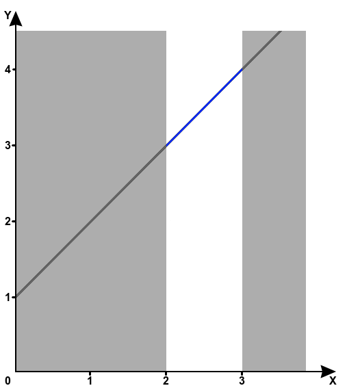
The lower bound equals 2, the upper bound equals 3, the Apply after calculation option is disabled
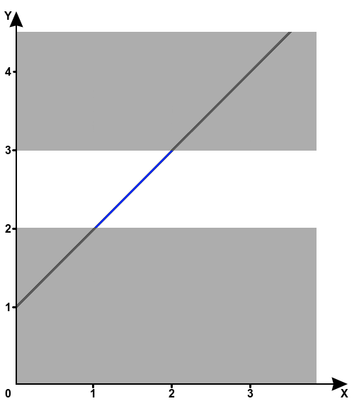
The lower bound equals 2, the upper bound equals 3, the Apply after calculation option is enabled
The principle of the calculation table operation
Sometimes, to understand the essence of a phenomenon, it’s better to go backward. If we know the precise formula Y=f(X), which relates the input and output values over the entire range, then there is no need to use the calculation table. It’s better to use the expression in the Parameter field instead. Let’s consider such a case.
Suppose that an input value is related to an output value by the Y=0.5⋅X2 formula.
Let’s take adc3 as a parameter. To describe such a formula in Wialon, insert the following expression into the Parameter field: const0.5*adc3^const2
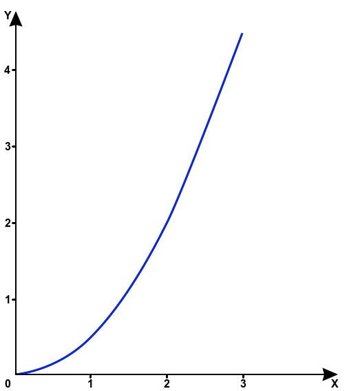
The chart of the Y=0.5⋅X2 function
But what if we don’t know the precise Y=f(X) formula? In this exact case, the calculation table will help us.
Suppose that we know the values of the measured value (it will be Y), and we can check what value the parameter will take in Wialon at those points (it will be X). Thus, you can get values, for example, at four points: (0; 0), (1; 0.5), (2; 2), (3; 4.5). Next, plot these points (X, Y) on the chart and connect them with red lines.
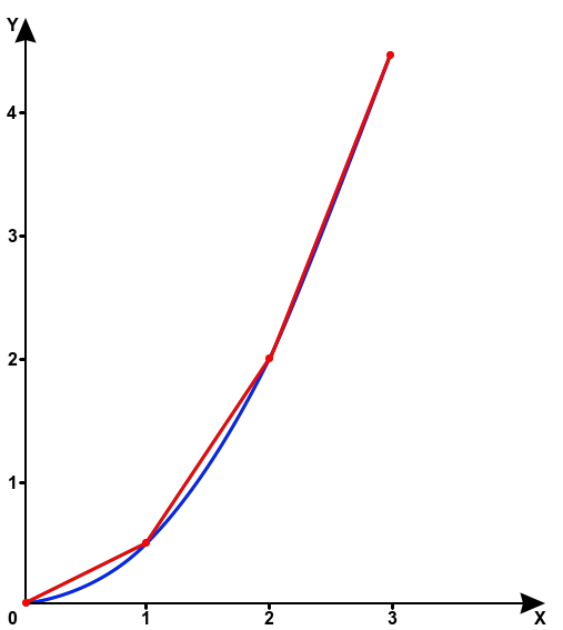
Reproduction of a part of the function Y=0.5⋅X2 by lines built on four points
It is easy to see that the result is close to that obtained by the formula, but there are still differences. In some cases, this accuracy will be sufficient, but if it is not enough, you can measure values at more points. The chart below shows an example for six points: (0; 0), (0.5; 0.125), (1; 0.5), (1.5; 1.125), (2; 2), (3; 4.5).
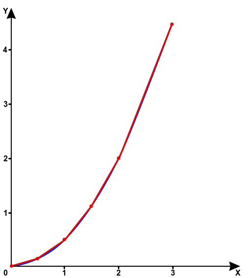
Reproduction of a part of the function Y=0.5⋅X2 by lines built on six points
From the considered example, we can draw the following conclusion: the relationship between X and Y can be described by a formula, but also it can be simplistically described with the help of several straight lines. This is the essence of using the calculation table.
Rationale and use cases
In this section, we will consider several cases where the calculation table saves the day.
The curve that describes the relationship between X and Y can be quite complex.
For example, using a fuel level sensor requires calibrating the fuel tank, and the shape of the chart built according to the calibration table will depend on the geometry of the tank, which is never ideal (it may have roundings, dents, internal stiffeners, and so on).
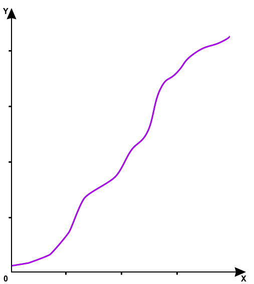
The chart based on the calibration table with small steps between measurements
It is problematic to describe such dependence in one formula. An easier way to describe this curve is to break it down into intervals where it behaves roughly like a straight line and determine the formulas for those lines. You can do it using XY pairs.
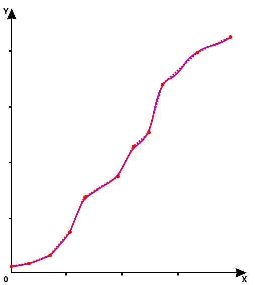
Reproduction of a complex curve by breaking it down into lines passing through eleven points
Also, sometimes the relationship between X and Y can vary over several intervals. To describe it, you need to use a system of several expressions, which cannot be done in the Parameter field in the sensor properties.
For example, some temperature sensors work as follows: X values in the range from 0 to 127 correspond to a positive temperature, and in the range from 128 to 255 — to a negative temperature. You will need a calculation table with two rows to handle such a case:
X=0; a=1; b=0
X=128; a=1; b=-256
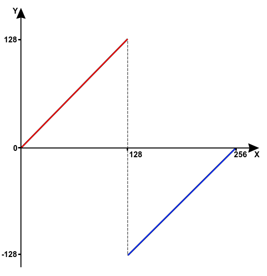
The temperature chart where higher parameter values correspond to negative temperatures
Digital sensors are another prime example of a situation where the relationship between X and Y varies over several intervals. For example, an ignition sensor can be created based on a voltage parameter, and this requires two conditions taken into account: Y=0 when X<14 and Y=1 when X≥14. As we already know, this cannot be done using an expression in the sensor properties. But on the Calculation Table tab, this will require only two lines:
X=0; a=0; b=0
X=14; a=0; b=1
In digital sensors, the slope coefficient always equals 0.
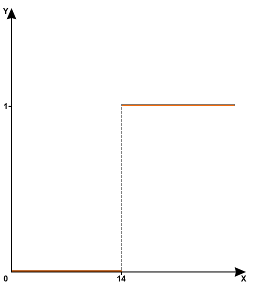
The ignition status chart depending on voltage
It’s Math Time
The article has already mentioned several times that the sensor ideally needs a formula for the relationship between X and Y, and we use the calculation table due to the lack of this formula. In fact, you can try to calculate such a formula, but to do this, you need to have an idea about numerical methods of analysis and the corresponding software. Unfortunately the result is likely to be intricate and hard to adjust in the future. To demonstrate this, we calculated an interpolation polynomial for the following 7 points: (0; 5), (400; 8), (1000; 22), (1850; 78), (2800; 160), (3600; 195), ( 4096; 200).
The result of polynomial interpolation, in this case, is as follows:
Y=1.78962834270398⋅10-19⋅X6-7.99064624017665⋅10-16⋅X5-4.83816855045549⋅10-12⋅X4+
+2.62803612257704⋅10-8⋅X3-1.24091655860425⋅10-5⋅X2+8.58707470047479⋅10-3⋅X+5
This formula can be entered in the Parameter field in the sensor properties taking into account the Wialon syntax, and it will work. The chart of such a function in the range from 0 to 4096 looks like this:
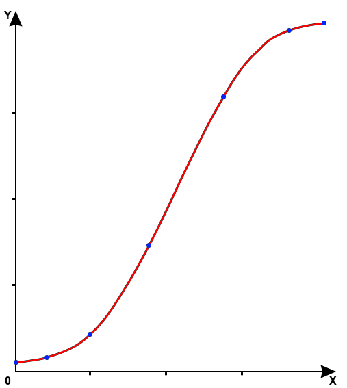
However, if the described dependence has a more complex form than shown in the chart above, you will have to take more points or use a different interpolation method. It might lead to the result that is even harder to understand. Therefore, linear interpolation, which is used in the calculation table in Wialon, looks very advantageous against this background since it is quite accurate and easy to use.